


9. What conclusions can we draw? Explain how this method could be used to assess the normality assumption (prior to conducting an ANOVA, perhaps).
***** ## Scenario: Male pattern heart disease? [Researchers](http://news.harvard.edu/gazette/2000/01.27/bald.html) selected a sample of 663 heart disease patients and a control group of 772 males not suffering from heart disease. Each subject was classified into one of 5 baldness categories:
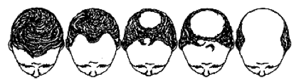
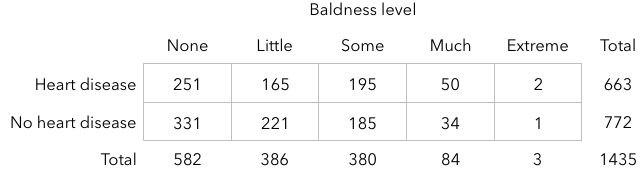
```{r, echo=FALSE} # Enter data baldness <- c(rep("none", 582), rep("little", 386), rep("some", 380), rep("much", 84), rep("extreme", 3)) disease <- c(rep("yes", 251), rep("no", 331), rep("yes", 165), rep("no", 221), rep("yes", 195), rep("no", 185), rep("yes", 50), rep("no", 34), rep("yes", 2), rep("no", 1)) baldheart <- data.frame(baldness, disease) ``` ```{r} # Mosaic plot mosaicplot(table(baldheart)) ``` 10. Do these results give us evidence that heart disease is associated with baldness? Calculate the relative risk of heart disease for each category of baldness. Then, calculate odds ratios.
Can we use a chi-square test to test for a relationship between heart disease in baldness? We can if we're able to derive our **expectations** for each cell.
### Expectation: Independence 11. Write out a null hypothesis for the relationship between heart disease and baldness.
12. What's it mean for two variables, A and B, to be **independent**?
13. If A and B are **independent**, P(A | B) = ___________ and P(A and B) = ____________________?
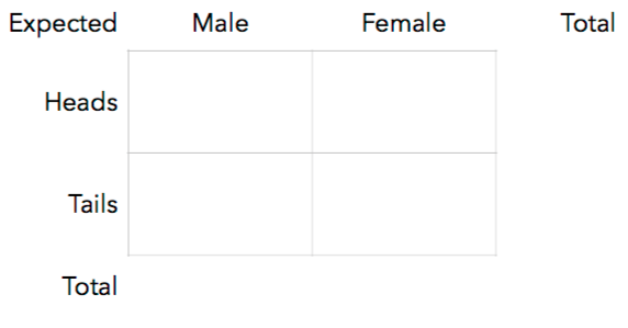
14. Suppose we’re interested in the relationship between gender and the result of a coin toss. We get 50 men and 50 women to each flip a coin and record the result. Assuming gender has no influence on the result of a coin toss, fill-in the **expectations** for each cell:
15. Derive a general formula to calculate the expectations for any rxc contingency table.
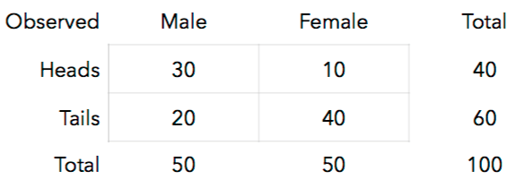
Suppose we conduct this experiment and get the following results:
#### Fisher's Exact Test
16. Look at the top-left cell. We expected 25 but observed 30. Using the [hypergeometric distribution](http://stattrek.com/online-calculator/hypergeometric.aspx), calculate the probability of observing 30 or more males flipping heads if gender and coin toss results are independent.
We can conduct this test (**Fisher's Exact Test**) in R: ```{r} # P(30 or more heads) = 1 - P(29 or fewer heads), where # m = 40 heads in the population # n = 60 tails in the population # k = 50 chosen for males 1 - phyper(29, 40, 60, 50, lower.tail=TRUE) # Enter the data for Fisher's Test coin <- c(rep("heads", 40), rep("tails", 60)) gender <- c(rep("male", 30), rep("female", 10), rep("male", 20), rep("female", 40)) coingender <- data.frame(coin, gender) # Examine the data tally(coin ~ gender, margins = TRUE, data=coingender) # Fisher's test fisher.test(coingender$gender, coingender$coin, alternative="less") ```
You can see the results from Fisher's Exact Test match the calculation from the hypergeometric distribution. This method is more difficult to use with larger numbers (or when our table isn't a 2x2 table). #### Chi-square test for independence Since we have expected and observed observations for categorical variables, we could also calculate a chi-square statistic. 17. Compute a chi-squared statistic and [estimate a p-value](http://lock5stat.com/statkey/theoretical_distribution/theoretical_distribution.html#chi). How many degrees-of-freedom does your test statistic have?
We can conduct this **chi-square test for independence** in R: ```{r} # Our data are still stored in the "coingender" data.frame # We use chisq.test(x, y) to run the test chisq.test(coingender$gender, coingender$coin, correct=FALSE) # We can estimate the p-value with randomization-based methods chisq.test(coingender$gender, coingender$coin, simulate.p.value=TRUE, B=5000) ```
### So... heart disease and baldness? Let's enter our heart disease / baldness data into R and run both Fisher's Exact Test and a Chi-square Test for Independence: ```{r} # Enter data baldness <- c(rep("none", 582), rep("little", 386), rep("some", 380), rep("much", 84), rep("extreme", 3)) disease <- c(rep("yes", 251), rep("no", 331), rep("yes", 165), rep("no", 221), rep("yes", 195), rep("no", 185), rep("yes", 50), rep("no", 34), rep("yes", 2), rep("no", 1)) baldheart <- data.frame(baldness, disease) # Check for entry errors tally(disease ~ baldness, margins = TRUE, data=baldheart) # Run Fisher's Exact Test fisher.test(baldheart$baldness, baldheart$disease, alternative="less") # Chi-square test for independence chisq.test(baldheart$baldness, baldheart$disease, correct=FALSE) # We can estimate the p-value with randomization-based methods chisq.test(baldheart$baldness, baldheart$disease, simulate.p.value=TRUE, B=5000) ```
18. Based on these results, what conclusions can you make?
***** ## Chi-squared tests - notes and warnings ### Conditions of the chi-square test One problem with the chi-square test is that the sampling distribution of the test statistic we calculate has an *approximate* chi-square distribution. With larger sample sizes, the approximation is good enough. With smaller sample sizes, however, p-values estimated from the chi-square distribution can be inaccurate. This is why many textbooks recommend you only use chi-square tests when the expected frequencies in each cell are **at least 5**. Even with large overall sample sizes, expected cell frequencies below 5 result in a loss of statistical power. When you have cells with less than 5 observations, you can: • Use Fisher's Exact Test • Use a likelihood ratio test (like the g-test we'll see in a bit) • Merge cells into larger bins to ensure observed frequencies are at least 5 Another condition of the chi-square test is **independence**. All observations must contribute to only one cell of the contingency table. You cannot use chi-square tests on repeated-measures designs.
### Effect sizes If you have a large sample size, the chi-square test will produce a low p-value... even if the difference in proportions is small. It's imperative that whenever you analyze contingency tables, you calculate some sort of effect size. You could calculate relative risk or odds ratios to give an estimate of the differences among categories.
### Yates's Correction When you have a 2x2 contingency table, the chi-square test (with one degree of freedom) tends to produce p-values that are too low (i.e., it makes Type I errors). One suggestion to address this issue is **Yates's continuity correction**. Yates's correction simply has you subtract 0.5 from the absolute value of the deviation in the numerator of our chi-square test statistic: $\chi _{\textrm{Yates}}^{2}=\frac{\left ( \left | O_{i}-E_{i} \right |-0.5 \right )^{2}}{E_{i}}$ This correction lowers our chi-square test statistic, thereby yielding a higher p-value. Although this may seem like a nice solution, there is evidence that this correction **over-corrects** and produces chi-square values that are too small. If you want to use Yates's correction in R, you simply tell R that `correct=TRUE`: ```{r} # Chi-square test for that baldness data chisq.test(baldheart$baldness, baldheart$disease, correct=TRUE) ```
### Likelihood ratio tests (G-test) An alternative to the chi-square test (that happens to produce results similar to the chi-square test) is the **G-test**. The G-test is an example of a **likelihood ratio test (LRT)**. We'll see other likelihood ratio tests later in the course. For now, let's conduct an LRT on a simple dataset. #### Scenario: Graduating from college Suppose you hypothesize 75% of St. Ambrose students graduate within 6 years. You then collect a sample of 1000 students and find 770 of them graduated within 6 years. You can think of this data as frequencies across two cells: 770 (graduated) and 230 (did not). With this, we could calculate a chi-square goodness-of-fit test: ```{r} # Input data graduated <- c(770, 230) # Input probabilities probabilities <- c(.75, .25) # Run the test chisq.test(graduated, p = probabilities) ```
We could also calculate the likelihood of observing this data under our hypothesis. If we think of each student as an independent trial with two possible outcomes (1 = graduated; 0 = did not), we can use the binomial distribution. We want to calculate **P(X = 770)** under a binomial distribution with **n = 1000 trials** and **p = 0.75** (our hypothesized value). Let's store this likelihood as `null`: ```{r} # P(X = 770) in binomial distribution with n=1000, p=0.75 null <- dbinom(770, size=1000, prob=0.75) null ```
Now let's an alternative hypothesis that the true proportion of students who graduate is 77%. We'll store this result as `alternative`: ```{r} # P(X = 770) in binomial distribution with n=1000, p=0.77 alternative <- dbinom(770, size=1000, prob=0.77) alternative ```
From these results, we'd conclude the data we obtained were more likely to be obtained if the true proportion of St. Ambrose students that graduate within 6 years is 77%. Let's take the ratio of the null likelihood to the alternative likelihood: ```{r} # Likelihood ratio LR <- null / alternative LR ```
This ratio will get smaller as the observed results get further away from our null hypothesis. If we take the natural log of this ratio and multiply it by -2, we get the *log-likelihood* (or **G-statistic**). $G=-2\textrm{ln}\frac{L_{\textrm{null}}}{L_{\textrm{alternative}}}$ We multiply by -2 and take the natural log because it results in a test statistic that approximates a chi-square distribution. Let's calculate this statistic for our graduation example and determine its likelihood from a chi-square distribution: ```{r} # Calculate G-statistic G <- -2 * log(LR) G # Compare it to chi-square distribution with df = 2-1 pchisq(G, df=1, lower.tail=FALSE) ```
For this simple example, our p-value is 0.140. From this, we have very little evidence to support the belief that 77% of students graduate from St. Ambrose within 6 years.
Calculating the G-statistic can be tedious. Thankfully, there's an easier formula to use (based on the fact that in the ratio of likelihoods, a lot of stuff cancels out): $G=2\sum_{i=1}^{c}\left [ O_{i}-\textrm{ln}\frac{O_{i}}{E_{i}} \right ]$
The G-test can also be used to test for independence. You can see how to [conduct this test in R here](http://rcompanion.org/rcompanion/b_04.html).
#### G-test vs. Chi-square test Since both the G-test and the chi-squared test can be used for both goodness-of-fit and independence, which test should you use? It depends. The G-test is more flexible and can be used for more elaborate (and additive) experimental designs. The chi-square test, on the other hand, is more easily understood and explained. The G-test uses the multinomial distribution in its calculation, whereas the chi-square test provides only an approximation.
***** # Your turn 19. Criminologists have long debated whether there is a relationship between weather conditions and the incidence of violent crime. The article *Is There a Season for Homocide?* (Criminology, 1988: 287-296) classified 1361 homicides according to season, resulting in table displayed below. Conduct a chi-square goodness-of-fit test (and the randomization-based chi-square test) to determine if seasons are associated with different numbers of violent crimes.

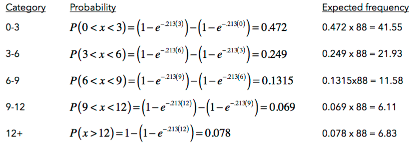
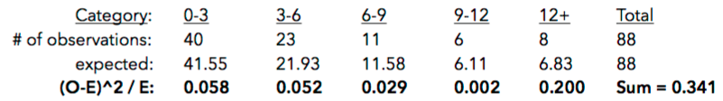
20. You may remember the dataset we analyzed in [lesson #3](http://bradthiessen.com/html5/stats/m301/lab3.html) regarding the amount of weight lost by subjects on various diets (e.g., Atkins, WeightWatchers). Prior to analyzing that data, we tested the homogeneity of variance assumption with Levene's test. Let's test for normality using a chi-square goodness-of-fit test.
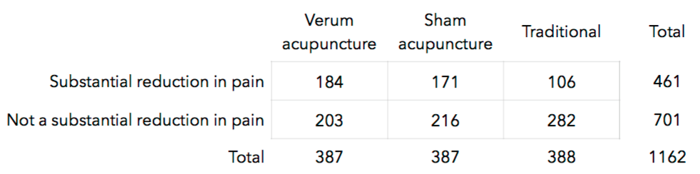
21. Is acupuncture effective in reducing pain? A [2007 study](http://www.ncbi.nlm.nih.gov/pubmed/17893311) looked at 1,162 patients with chronic lower back pain. The subjects were randomly assigned to one of 3 groups:
• **Verum acupuncture** practiced according to traditional Chinese principles,
• **Sham acupuncture** where needles were inserted into the skin but not at acupuncture points,
• **Traditional** (non-acupuncture) therapy consisting of drugs, physical therapy, and exercise.
Results are displayed in the table below.
**(a)** Calculate the probability that an individual undergoing verum acupuncture experienced a substantial reduction in pain.
**(b)** Calculate this same probability for the subjects in the traditional group.
**(c)** Calculate and interpret the ratio of the two probabilities you just calculated.
**(d)** Run a chi-square test for independence and interpret the result.
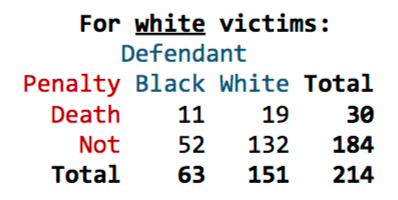
22. The table displayed below shows the number of black and white defendants sentenced to death in the 1960s-70s for murdering a white victim. As you can see, a higher proportion of black defendants were sentenced to death.
**(a)** Run Fisher's Exact Test to calculate the likelihood of observing results as or more extreme than these results if, in fact, race and the death penalty were independent.
**(b)** Run a chi-square test for independence.
***** # Publishing your solutions When you're ready to try the **Your Turn** exercises: - Download the appropriate [Your Turn file](http://bradthiessen.com/html5/M301.html). - If the file downloads with a *.Rmd* extension, it should open automatically in RStudio. - If the file downloads with a *.txt* extension (or if it does not open in RStudio), then: - open the file in a text editor and copy its contents - open RStudio and create a new **R Markdown** file (html file) - paste the contents of the **Your Turn file** over the default contents of the R Markdown file. - Type your solutions into the **Your Turn file**. - The file attempts to show you *where* to type each of your solutions/answers. - Once you're ready to publish your solutions, click the **Knit HTML** button located at the top of RStudio:
 - Once you click that button, RStudio will begin working to create a .html file of your solutions.
- It may take a minute or two to compile everything, especially if your solutions contain simulation/randomization methods
- While the file is compiling, you may see some red text in the console.
- When the file is finished, it will open automatically.
- If the file does not open automatically, you'll see an error message in the console.
- Send me an [email](mailto:thiessenbradleya@sau.edu) with that error message and I should be able to help you out.
- Once you have a completed report of your solutions, look through it to see if everything looks ok. Then, send that yourturn.html file to me [via email](mailto:thiessenbradleya@sau.edu) or print it out and give it to me.
- Once you click that button, RStudio will begin working to create a .html file of your solutions.
- It may take a minute or two to compile everything, especially if your solutions contain simulation/randomization methods
- While the file is compiling, you may see some red text in the console.
- When the file is finished, it will open automatically.
- If the file does not open automatically, you'll see an error message in the console.
- Send me an [email](mailto:thiessenbradleya@sau.edu) with that error message and I should be able to help you out.
- Once you have a completed report of your solutions, look through it to see if everything looks ok. Then, send that yourturn.html file to me [via email](mailto:thiessenbradleya@sau.edu) or print it out and give it to me.
Sources:
[Explanation of Benford's Law](http://www.datagenetics.com/blog/march52012/index.html)
[Chi-squared randomization applet](http://lock5stat.com/statkey/advanced_goodness/advanced_goodness.html)
[Chi-squared distribution applet](http://lock5stat.com/statkey/theoretical_distribution/theoretical_distribution.html#chi)
[List of categorical analysis methods](https://en.wikipedia.org/wiki/List_of_analyses_of_categorical_data)
This document is released under a [Creative Commons Attribution-ShareAlike 3.0 Unported](http://creativecommons.org/licenses/by-sa/3.0) license.