---
title: "Post-hoc tests"
author: "Lesson 4"
output:
html_document:
css: http://www.bradthiessen.com/batlab2.css
highlight: pygments
theme: spacelab
toc: yes
toc_depth: 5
fig_width: 5.6
fig_height: 4
---
```{r message=FALSE, echo=FALSE}
# Load the mosaic package
library(mosaic)
```
*****
## Scenario: Job interviews
Does having a disability influence how others perceive you perform on a job interview? If so, is the effect positive or negative?

To study this, researchers prepared five videotaped job interviews using the same two male actors for each. A set script was designed to reflect an interview with an applicant of average qualifications. The tapes differed only in that the applicant appeared with a different handicap:
• In one, he appeared in a **wheelchair**
• In a second, he appeared on **crutches**
• In a third, his **hearing** was impaired
• In a fourth, he appeared to have one leg **amputated**
• In a fifth, he appeared to have **no disability**
70 undergraduate students from an American university were randomly assigned to view the tapes, 14 to each tape. After viewing the tape, each subject rated the qualifications of the applicant on a 0-10 point scale.
Our primary questions are:
• Is having a disability associated with higher or lower interview scores?
• Do permanent disabilities (amputee, hearing, wheelchair) receive higher/lower scores than temporary disabilities (crutches)?
*****
## Data, assumptions, ANOVA
Here's a summary of the interview scores given by the 70 undergraduate students:
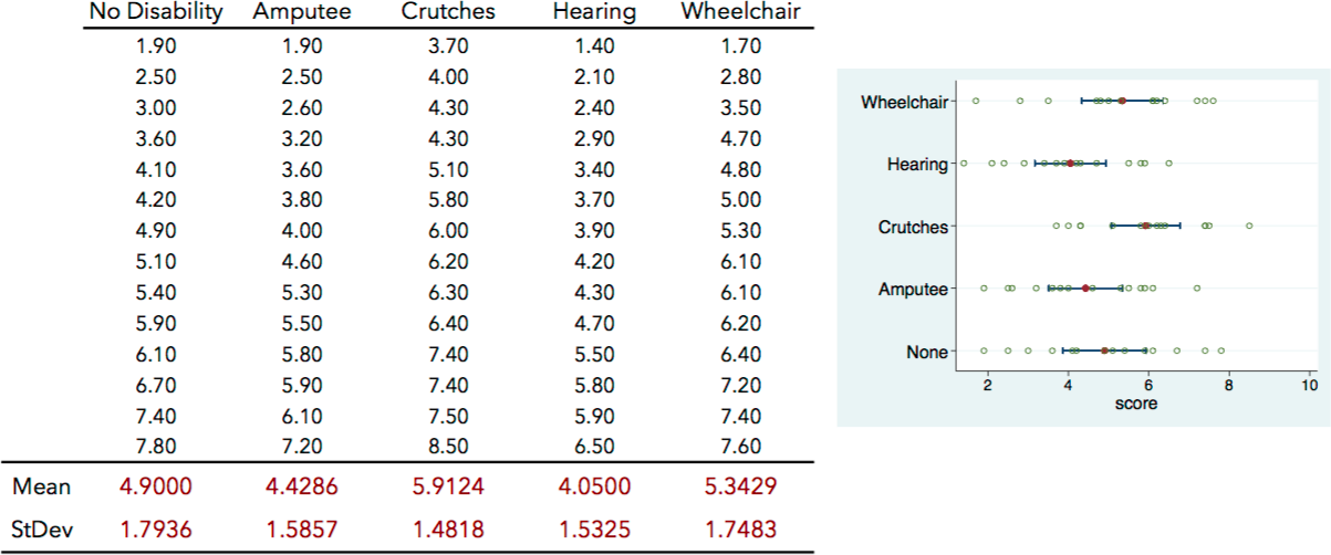
Let's download this data, visualize it, and test some assumptions for an ANOVA.
```{r}
# Download data from my website and store it as "interviews"
interviews <- read.csv("http://www.bradthiessen.com/html5/data/disability.csv")
# See the first several rows of data to get a sense of the contents
head(interviews)
# Stripplot
stripplot(score ~ disability, data=interviews, jitter.data = TRUE,
xlab = "anxiety", cex=1.3, col="steelblue", aspect="1", pch=20)
# Boxplot
bwplot(score ~ disability, data=interviews, col="steelblue", xlab="Group", ylab="scores",
par.settings=list(box.rectangle=list(lwd=3), box.umbrella=list(lwd=3)))
# Error bars showing mean and standard errors
# I need to load the ggplot2 library to generate this plot
library(ggplot2)
ggplot(interviews, aes(disability, score)) +
stat_summary(fun.y = mean, geom = "point") +
stat_summary(fun.y = mean, geom = "line", aes(group = 1),
colour = "Blue", linetype = "dashed") +
stat_summary(fun.data = mean_cl_boot, geom = "errorbar", width = 0.2) +
labs(x = "Disability", y = "Interview score")
# Run Shapiro-Wilk test for normality
# I run the test for each disability and then print all p-values
a <- round(shapiro.test(interviews$score[interviews$disability=="Amputee"])$p.value,3)
c <- round(shapiro.test(interviews$score[interviews$disability=="Crutches"])$p.value,3)
h <- round(shapiro.test(interviews$score[interviews$disability=="Hearing"])$p.value,3)
n <- round(shapiro.test(interviews$score[interviews$disability=="none"])$p.value,3)
w <- round(shapiro.test(interviews$score[interviews$disability=="Wheelchair"])$p.value,3)
paste("Amputee: p =", a, ". Crutch: p =", c, ". Hear: p =", h, ". none: p =", n, ". W-chair: p =", w)
# Levene's test for equal variances
leveneTest(score ~ disability, data=interviews)
```
1. Evaluate the assumptions necessary to conduct an ANOVA on this dataset.
Let's run the ANOVA:
```{r}
# Run the analysis of variance (aov) model
model <- aov(score ~ disability, data=interviews)
# Show the output in an ANOVA summary table
anova(model)
```
2. From this, what can we conclude? Calculate and interpret an effect size.
Even though the p-value indicates it's unlikely we would have observed this data if the group population means were equal, the ANOVA does not allow us to identify **which** group means differ from one another.
Since the questions of interest in this study are related to comparisons among specific group means, we need to derive some methods to do just that. We'll classify these *post-hoc* methods as:
• Pairwise-comparisons
• Flexible comparisons (contrasts)
*****
## Pairwise comparisons
Since we found a *statistically significant* result with our ANOVA, why don't we just compare each pair of group means using t-tests?
3. Calculate the probability of making at least one Type I error if we conducted t-tests on all pairs of group means in this study (using $\alpha =0.05$ for each t-test).
4. If we wanted the overall Type I error rate for all pairwise t-tests combined to be $\alpha =0.05$, what could we do?
### Bonferroni correction
This is the idea behind the **Bonferroni correction.** If we want to maintain an overall Type I error rate, we need to divide $\alpha$ for each test by the number of tests we want to conduct:
**Bonferroni correction**: $\alpha_{\textrm{each test}}=\frac{\alpha_{\textrm{overall}}}{\textrm{\# of tests}}$.
So, for example, if we wanted to conduct 10 t-tests and maintain an overall Type I error rate of 0.05, we would need to use $\alpha_{\textrm{each test}}=0.005$.
Instead of adjusting the Type I error rate for each test, we could correct the p-values **after** running the t-tests. To do this, we would use:
$\left (\textrm{p-value from each test} \right )\left ( \textrm{\# of tests to be conducted} \right )$
Let's see the Bonferroni correction in action. Remember, the p-value from the ANOVA we conducted earlier implies at least one of our group means differs from the others. *(This isn't exactly true. It actually tells us at least one linear combination of our group means will differ significantly from zero)*
We'll have R run all the pairwise t-tests to compare pairs of group means. First, we'll have R run t-tests with no adjustment to the p-values. Then, we'll adjust the p-values with the Bonferroni correction.
```{r}
# Pairwise t-tests with no adjustment
with(interviews, pairwise.t.test(score, disability, p.adjust.method="none"))
# Pairwise t-tests with Bonferroni correction on the p-values
# Verify the p-values increase by a factor of 10 (in this example)
with(interviews, pairwise.t.test(score, disability, p.adjust.method="bonferroni"))
```
5. From this output (using the Bonferroni correction), what conclusions can we make? Which disability group means differ from others?
6. Remember, the Bonferroni correction increases the magnitude of our p-values (by lowering the Type I error rate). This makes it **less likely** to reject a null hypothesis and conclude a pair of group means differs from one another. What does that do to the **power** of our statistical tests? Identify a drawback with the Bonferroni correction.
7. Should we only conduct a post-hoc test (like pairwise t-tests with the Bonferroni correction) when our overall ANOVA produces a statistically significant result? Explain.
Because Bonferroni's correction is *conservative* (and can struggle to find mean differences that actually exist), several other post-hoc strategies have been developed.
### Holm's method
One alternative strategy that's relatively easy to explain is **Holm's method**. You first conduct all pairwise t-tests to obtain a p-value from each test. Then, you rank order those p-values from largest to smallest. For our data, the ranked order of our (uncorrected) p-values is:
- 1: Hearing vs Amputee (p=0.5418)
- *(I'll skip 2 through 5)*
- 6: Wheelchair vs Amputee (p=0.1433)
- 7: None vs Crutches (p=0.1028)
- 8: Hearing vs Wheelchair (p=0.0401)
- 9: Crutches vs Amputee (p=0.0184)
- 10: Crutches vs Hearing (p=0.0035)
We then correct each of those p-values by multiplying the p-value by its rank:
- 1: Hearing vs Amputee (p=0.5418 multiplied by 10 takes us above 1.000)
- *(I'll skip 2 through 5)*
- 6: Wheelchair vs Amputee (p=0.1433 multiplied by 6 = 0.860)
- 7: None vs Crutches (p=0.1028 multiplied by 7 = 0.719)
- 8: Hearing vs Wheelchair (p=0.0401 multiplied by 8 = 0.321)
- 9: Crutches vs Amputee (p=0.0184 mutiplied by 9 = 0.165)
- 10: Crutches vs Hearing (p=0.0035 multiplied by 10 = 0.035)
Notice that for the smallest p-value, this method is exactly the same as the Bonferroni correction. In subsequent comparisons, however, the p-value is **corrected only for the remaining number of comparisons**. This makes it more likely to find a difference between a pair of group means.
Let's have R calculate the pairwise tests using Holm's method:
```{r}
# Holm's method
with(interviews, pairwise.t.test(score, disability, p.adjust.method="holm"))
```
### Other post-hoc methods
There are many more post-hoc methods (e.g., Hochberg's False Discovery Rate, Tukey's Honestly Significant Difference, Dunnett's method) that we simply don't have time to investigate. It is important, though, that you get a sense for which methods perform best.
As you learned in a previous statistics class, the Type I error rate is linked to the statistical power of a test. If we increase the probability of making a Type I error, the power declines (and vice versa). Because of this, it's important that post-hoc methods control the overall Type I error rate without sacrificing too much power.
Bonferroni's correction and Tukey's HSD control the Type I error rate well, but they lack statistical power. Bonferroni's correction has more power when testing a small number of comparisons, while Tukey's HSD performs better with a larger number of comparisons. Holm's method is more powerful than both Bonferroni and Tukey (and Hochberg's method is more powerful still).
Each of these methods, however, performs poorly if the population group variances differ *and* the sample sizes are unequal. If you have an *unequal sample sizes* and *unequal variances*, you should probably use a robust post-hoc comparison method.
In case you're interested, here's the code to conduct a Tukey's HSD:
```{r}
# Conduct the post-hoc test
TukeyHSD(model, conf.level=.95)
# See a plot of the confidence intervals for each pairwise mean difference
plot(TukeyHSD(model))
```
*****
## Scheffe method for flexible comparisons (contrasts)
The previous methods allow us to compare pairs of means. Sometimes, as in this scenario, we'll want more flexibility. For example, think about the key questions in this study:
- Is having a disability associated with higher or lower interview scores?
- Do permanent disabilities (amputee, hearing, wheelchair) receive higher/lower scores than temporary disabilities (crutches)?
To address these questions, we'll need to compare **linear combinations** of group means:
- The no disability group vs. the 4 other groups.
- Permanent disabilities (amputee, hearing, wheelchair) vs. temporary (crutches, none).
Let's focus on that first contrast (no disability vs. the 4 disability groups). To compare this linear combination of means, we can use the **Scheffe method**.
With the Scheffe method, we first need to calculate our contrast of interest by choosing weights in our linear combination:
**Contrast** (linear combination of means): $\psi =\sum_{a=1}^{a}c_{a}\mu _{a}=c_{1}\mu _{1}+c_{2}\mu _{2}+c_{3}\mu _{3}+c_{4}\mu _{4}+c_{5}\mu _{5}, \ \ \ \textrm{where} \ \sum c_{a}=0$
8. Calculate an estimate of the contrast to compare the **none** group mean with a combination of the other 4 group means. Under a true null hypothesis, the expected value of this contrast would equal what?
Our contrast isn't zero, but we wouldn't expect any contrast calculated from real data to equal zero. Even if the population values of our group means were identical, we'd expect our sample group means to differ and our sample contrast to be nonzero.
So our task is to determine the likelihood of observing a contrast as or more extreme than the one we calculated (assuming the null hypothesis is true). To do this, we need to derive the sampling distribution of our contrast.
Recall the general form of a t-test. We may be able to use the t-distribution to determine the likelihood of our contrast:
$t=\frac{\textrm{observed}-\textrm{hypothesized}}{\textrm{standard error}}=\frac{\hat{\psi }-0}{\textrm{SE}_{\psi }}$
If this works, we only need to derive the standard error of a contrast. Then, we’d know the distribution of our sample contrast and we could estimate its likelihood.
To derive the standard error of a contrast, we need to remember two properties of variances:
- $\textrm{var}\left ( ax \right )=a^{2}\textrm{var}\left ( x \right )$.
- If X and Y are independent, then: $\textrm{var}\left ( X+Y \right )=\textrm{var}\left ( X \right )+\textrm{var}\left ( Y \right )$
With these two facts, we can calculate the variance of our contrast:
$\textrm{var}\left ( \hat{\psi} \right )=\textrm{var}\left ( c_{1}\overline{X}_{1} \right )+\textrm{var}\left ( c_{2}\overline{X}_{2} \right )+\textrm{var}\left ( c_{3}\overline{X}_{3} \right )+\textrm{var}\left ( c_{4}\overline{X}_{4} \right )+\textrm{var}\left ( c_{5}\overline{X}_{5} \right )$
$\textrm{var}\left ( \hat{\psi} \right )=c_{1}^{2}\textrm{var}\left ( \overline{X}_{1} \right )+c_{2}^{2}\textrm{var}\left ( \overline{X}_{2} \right )+c_{3}^{2}\textrm{var}\left ( \overline{X}_{3} \right )+c_{4}^{2}\textrm{var}\left ( \overline{X}_{4} \right )+c_{5}^{2}\textrm{var}\left ( \overline{X}_{5} \right )$
We now need one other fact about the variance of a mean: $\textrm{var}\left ( \overline{X} \right )=\frac{\sigma _{x}^{2}}{n}$
$\textrm{var}\left ( \hat{\psi} \right )=c_{1}^{2}\frac{\sigma _{1}^{2}}{n_{1}}+c_{2}^{2}\frac{\sigma _{2}^{2}}{n_{2}}+c_{3}^{2}\frac{\sigma _{3}^{2}}{n_{3}}+c_{4}^{2}\frac{\sigma _{4}^{2}}{n_{4}}+c_{5}^{2}\frac{\sigma _{5}^{2}}{n_{5}}$
If we're going to assume the group variances are equal (which we already assumed in our ANOVA), we have:
$\textrm{var}\left ( \hat{\psi} \right )=\sum \frac{c_{a}^{2}}{n_{a}}\sigma _{x}^{2}$
Finally, we know MSE is our best estimate of the pooled standard deviation of our groups, so we can substitute:
$\textrm{var}\left ( \hat{\psi} \right )=\textrm{MS}_{\textrm{E}}\sum \frac{c_{a}^{2}}{n_{a}}$
That's the standard error of our contrast. We can now substitute this into our t-statistic:
$t=\frac{\textrm{observed}-\textrm{hypothesized}}{\textrm{standard error}}=\frac{\hat{\psi }-0}{\textrm{SE}_{\psi }}=\frac{\hat{\psi }-0}{\sqrt{\textrm{MS}_{\textrm{E}}\sum \frac{c_{a}^{2}}{n_{a}}}} \sim\sqrt{\left ( a-1 \right )F}$
9. Use what was just derived to estimate the p-value of our contrast of interest. What conclusions can we make?
Now let's try to calculate this Scheffe statistic in R. Remember, we're comparing the mean of the "no disability" group to the combination of the 4 disability group means:
```{r}
# Create vector of contrast coefficients
coeff <- c(-1/4,-1/4,-1/4,1,-1/4)
# Store group means as mm
mm <-mean(score ~ disability, data=interviews)
# Store group sample sizes as nn
nn <- tapply(interviews$score, interviews$disability, length)
# Calculate contrast (psi)
psi <- sum(coeff*mm)
# Calculate standard error of contrast
# First, run the ANOVA to get the mean squares
omnianova <- anova(aov(score ~ disability, data=interviews))
# Then, store mean square error as MSE
MSE <- omnianova$`Mean Sq`[2]
# Finally, calculate the SE of our psi
SEpsi <- sqrt(MSE) * sqrt( sum((coeff^2)/nn) )
# Calculate our test statistic (psi / std. error)
PSIoverSE <- psi / SEpsi
# Find critical value
# Choose alpha
alpha = 0.05
# sqrt(a-1) x sqrt(F)
cv <- sqrt(omnianova$Df[1]) * sqrt(qf(1-alpha, omnianova$Df[1], omnianova$Df[2]))
# Paste results
paste("observed test.stat =", round(PSIoverSE,4), ". Critical value =", round(cv,4))
```
We can get the same result with another contrast:
```{r}
coeff <- c(-1,-1,-1,4,-1)
mm <-mean(score ~ disability, data=interviews)
nn <- tapply(interviews$score, interviews$disability, length)
psi <- sum(coeff*mm)
omnianova <- anova(aov(score ~ disability, data=interviews))
MSE <- omnianova$`Mean Sq`[2]
SEpsi <- sqrt(MSE) * sqrt( sum((coeff^2)/nn) )
PSIoverSE <- psi / SEpsi
alpha = 0.05
cv <- sqrt(omnianova$Df[1]) * sqrt(qf(1-alpha, omnianova$Df[1], omnianova$Df[2]))
paste("observed test.stat =", round(PSIoverSE,4), ". Critical value =", round(cv,4))
```
Because the observed test statistic is less than the critical value, we'd conclude that we do not have evidence that the mean of the no disability group differs from the mean of the combination of the disability groups.
10. Write out the contrast you would use to compare the **temporary** disabilities (none and crutches) to the **permanent** disabilities (amputee, hearing, and wheelchair).
Let's use the Scheffe method to compare this linear combination of group means:
```{r}
coeff <- c(-2,3,-2,3,-2)
mm <-mean(score ~ disability, data=interviews)
nn <- tapply(interviews$score, interviews$disability, length)
psi <- sum(coeff*mm)
omnianova <- anova(aov(score ~ disability, data=interviews))
MSE <- omnianova$`Mean Sq`[2]
SEpsi <- sqrt(MSE) * sqrt( sum((coeff^2)/nn) )
PSIoverSE <- psi / SEpsi
alpha = 0.05
cv <- sqrt(omnianova$Df[1]) * sqrt(qf(1-alpha, omnianova$Df[1], omnianova$Df[2]))
paste("observed test.stat =", round(PSIoverSE,4), ". Critical value =", round(cv,4))
```
11. From this, what conclusions can you make?
*****
# Your turn
```{r, echo=FALSE, message=FALSE}
# Load data
music <- read.csv("http://www.bradthiessen.com/html5/data/music.csv")
```
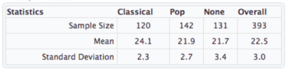
12. A [2003 study](http://eab.sagepub.com/content/35/5/712.abstract) investigated the effect of background music on the amount of money diners spend in restaurants. A British restaurant alternated among 3 types of background music -- **None** (silence), **Pop** music, and **Classical** music -- over the course of 18 days. Each type of music was played for 6 nights, with the order of the music being randomly determined.
The data from **N = 393** diners have been loaded in a data.frame called **music**. The variables are **MusicType** and **Amount** (the amount of money spent per person).
**(a)** The variances in amount spent for each type of music range from `r round(var(music$Amount[music$MusicType=="Classical"]),3)` (for Classical music) to `r round(var(music$Amount[music$MusicType=="None"]),3)` (for None). That means the largest variance of a treatment is only a little more than twice as big as the smallest variance. When I conduct a Levene's Test for equal variances (as displayed below), the p-value is **0.002**. Explain why the p-value for this test is so low for this dataset if the sample variances only differ by a factor of 2.
**(b)** Conduct an ANOVA to compare the average amount spent for the 3 types of music.
**(c)** Use the Bonferroni correction to test all pairs of group means.
**(d)** Use Holm's method to compare all pairs of group means.
**(e)** Write out all conclusions you can make about the effect of background music on the amount of money diners spend.
**(f)** Use Scheffe's method to compare no music (**None**) against the combination of **Classical** and **Pop** music.
**(g)** Write a conclusion.
```{r}
# Load data
music <- read.csv("http://www.bradthiessen.com/html5/data/music.csv")
# Means plot with standard error bars
ggplot(music, aes(MusicType, Amount)) +
stat_summary(fun.y = mean, geom = "point") +
stat_summary(fun.y = mean, geom = "line", aes(group = 1),
colour = "Blue", linetype = "dashed") +
stat_summary(fun.data = mean_cl_boot, geom = "errorbar", width = 0.2) +
labs(x = "Music Type", y = "Money Spent")
# Levene's test for equal variances
leveneTest(Amount ~ MusicType, data=music)
```
*****
# Publishing your solutions
When you're ready to try the **Your Turn** exercises:
- Download the appropriate [Your Turn file](http://bradthiessen.com/html5/M301.html).
- If the file downloads with a *.Rmd* extension, it should open automatically in RStudio.
- If the file downloads with a *.txt* extension (or if it does not open in RStudio), then:
- open the file in a text editor and copy its contents
- open RStudio and create a new **R Markdown** file (html file)
- paste the contents of the **Your Turn file** over the default contents of the R Markdown file.
- Type your solutions into the **Your Turn file**.
- The file attempts to show you *where* to type each of your solutions/answers.
- Once you're ready to publish your solutions, click the **Knit HTML** button located at the top of RStudio:  - Once you click that button, RStudio will begin working to create a .html file of your solutions.
- It may take a minute or two to compile everything, especially if your solutions contain simulation/randomization methods
- While the file is compiling, you may see some red text in the console.
- When the file is finished, it will open automatically.
- If the file does not open automatically, you'll see an error message in the console.
- Send me an [email](mailto:thiessenbradleya@sau.edu) with that error message and I should be able to help you out.
- Once you have a completed report of your solutions, look through it to see if everything looks ok. Then, send that yourturn.html file to me [via email](mailto:thiessenbradleya@sau.edu) or print it out and give it to me.
- Once you click that button, RStudio will begin working to create a .html file of your solutions.
- It may take a minute or two to compile everything, especially if your solutions contain simulation/randomization methods
- While the file is compiling, you may see some red text in the console.
- When the file is finished, it will open automatically.
- If the file does not open automatically, you'll see an error message in the console.
- Send me an [email](mailto:thiessenbradleya@sau.edu) with that error message and I should be able to help you out.
- Once you have a completed report of your solutions, look through it to see if everything looks ok. Then, send that yourturn.html file to me [via email](mailto:thiessenbradleya@sau.edu) or print it out and give it to me.
Sources:
**Study**: Cesare, Tannenbaum, Dalessio (1990). Interviewers’ Decisions Related to Applicant Handicap Type and Rater Empathy. Human Performance, 3(3)
This document is released under a [Creative Commons Attribution-ShareAlike 3.0 Unported](http://creativecommons.org/licenses/by-sa/3.0) license.