---
title: "Repeated Measures & Experimental Design"
author: "Lesson 6"
output:
html_document:
css: http://www.bradthiessen.com/batlab2.css
highlight: pygments
theme: spacelab
toc: yes
toc_depth: 5
fig_width: 5.6
fig_height: 4
---
```{r message=FALSE, echo=FALSE}
# Load the mosaic package
library(mosaic)
```
*****
1. Fill-in-the-blanks:
In a one-way ANOVA, SStotal is partitioned into 2 components:
(1) _______________ (variance due to the treatment effect) and (2) _______________ (unexplained variance).
We divide SS by their df to get ____________ which represent ________________________________________.
We then calculate the ratio of those MS values and compare it to the _______________ distribution.
Under the null hypothesis, we expect this ratio to equal _______________.
If the null hypothesis is false, this ratio will be _________________________.
The power of a statistical test refers to ____________________________________________________________.
If we want to increase the power of our ANOVA, we could:
(a) ______________________________ our sample size,
(b) ______________________________ our alpha-level, or
(c) ______________________________ the size of MSE.
If MSE is small, our MSR will be ____________________ and we have a better chance of rejecting our null hypothesis.
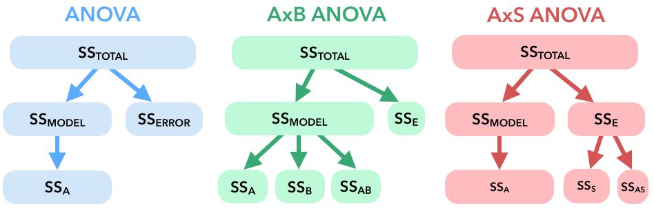
2. The following figures attempt to demonstrate how the total variation is partitioned under one-way, AxB, and AxS (repeated measures) ANOVA. Explain how the AxB and AxS work to increase the power of our test.
*****
## Scenario: Optimism
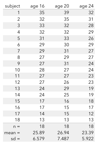
How optimistic are you? Are you more or less optimistic than you were when you were 16? To study this, 50 subjects were given an optimism test at age 16. These same subjects were give the same test at ages 20 and 24. A total of 18 subjects completed the survey at all 3 ages. The data for these 18 subjects is displayed below:
```{r}
# Load optimism data
optimism <- read.csv("http://www.bradthiessen.com/html5/data/opt.csv")
## Change subject and age to factor variables
optimism$age <-as.factor(optimism$age)
optimism$subject <-as.factor(optimism$subject)
## Summary of data
favstats(optimism ~ age, data=optimism)
## Some summary plots
densityplot(~optimism | age, data=optimism, lwd=2,
main="Optimism by age", layout=c(1,3))
## Levene's test
leveneTest(optimism ~ age, data=optimism)
```
### Incorrect analysis: one-way ANOVA
Let's pretend as though the data in this study come from 3 independent groups of subjects (and **not** the same subjects at 3 different ages). With this erroneous assumption, let's conduct a one-way ANOVA:
```{r}
# Summarize ("anova") the analysis ("aov")
anova(aov(optimism ~ age, data=optimism))
# Post-hoc tests with Holm's method
with(optimism, pairwise.t.test(optimism, age, p.adjust.method="holm"))
```
3. What conclusion would we make about optimism across the age groups? Calculate and interpret an effect size.
### Somewhat correct analysis: AxS ANOVA
The data in this study did **not** come from 3 independent groups. The scores are from the same 18 subjects measured 3 different times (at ages 16, 20, and 24). This is called a *repeated measures* design.
4. What are some advantages and disadvantages in designing this study for repeated measures?
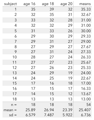
Before we conduct an AxS (repeated measures) ANOVA, let's calculate the mean optimism score for each of the 18 subjects in this study.
```{r}
# Mean optimism for each subject
mean(optimism ~ subject, data=optimism)
```
We can display those means alongside our data.
5. Let's construct a model for our data. In our dataset, why do optimism scores differ from others?
The **age effect** is what we're interested in estimating. When we analyzed the data with a one-way ANOVA, we treated all other sources of variation as unexplained error variance.
In an AxS design, we can partition this unexplained error variance further (by explaining some of it as individual subject differences).
We know some of the variation in optimism within and across the age groups is due to pre-existing individual differences. For example, subject #3 tends to be more optimistic than subject #18. If we can estimate these *subject-effects*, we can remove them from our unexplained error variance.
After estimating the age and subject effects, the only remaining variation would be due to the interaction between a subject and his or her age. Some people will become more optimistic over time, some will become less optimistic, and others will have other *paths*. This variation is still considered unexplained, because it includes other potential factors, too.
Let's take a look at the *paths* of our subjects across the age groups:
```{r}
# Profile plots (optimism by subject at each age)
interaction.plot(x.factor=optimism$age, trace.factor=optimism$subject,
response=optimism$optimism,
fun=mean, type="b", legend=F,
ylab = "Mean optimism score", xlab = "Age group")
# This plot looks a little nicer. It uses the ggplot2 package
library(ggplot2)
# Here's the syntax
ggplot(data = optimism, aes(x = age, y = optimism, group = subject)) +
ggtitle("Optimism by age") +
ylab("optimism") + geom_line()
```
6. Based on the profile plots, do you think we'll find a significant subject effect? In other words, do the subjects seem to be consistent across age groups?
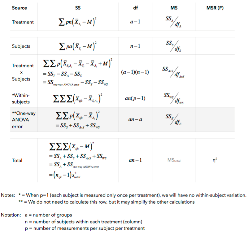
#### Formulas for AxS ANOVA
To calculate an AxS ANOVA by hand, you could use the following formulas:
We can calculate everything in R:
```{r}
# AxS ANOVA
# We specify the error term as "subjects nested within age groups"
axs <- aov(optimism ~ age + Error(subject/age), data=optimism)
# We have to use "summary" (and not "anova") to get the summary table
summary(axs)
```
Here are the same results calculated by hand:
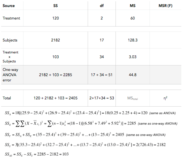
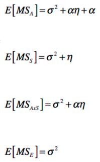
7. Which mean square ratios do we calculate? To help answer this, take a look at the expected value of our mean square terms. If we're interested in the effect of age on optimism, which mean square ratio should we calculate?
8. Calculate the appropriate mean square ratio and compare it to the output from R. Explain why your conclusion from the AxS ANOVA differs from your conclusion from the one-way ANOVA. Then, calculate an effect size for the effect of age on optimism.
9. Calculate an effect size for the subject effect. What proportion of variation in optimism is due to the individual subjects? Was it worthwhile to conduct this study as a repeated measures design? Explain.
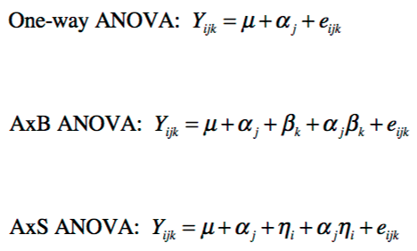
10. The models for one-way, AxB, and AxS ANOVA analyses are displayed below. Interpret each piece of the model for the AxS ANOVA.
*****
## Other experimental designs (GwT)
Suppose we're interested in the the effectiveness of statistics textbooks. If we sample 3 classrooms and randomly assign them to use one of 3 different textbooks, our data could look like this:
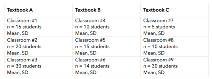
11. At first glance, it might seem as though we could analyze this data with a one-way ANOVA (or perhaps an AxB ANOVA). Explain why we should **not** use a one-way or AxB ANOVA to analyze this data. Which condition has been violated?
12. How many independent observations do we have in our dataset: 9 or 150?
Let's look at a different dataset. In Iowa, local governments can be organized in several ways (*e.g., mayor and council with all officers elected at large; mayor elected at large with council members elected by district; council members elected by district and mayor elected from within the council; variations of these organizational types with and without a hired city manager; etc.*).
A political scientist wanted to investigate whether some organizations of local governments result in more *content* citizens than others. He identified 4 types of government (A1, A2, A3, A4) and interviewed citizens regarding their satisfaction with the local government's responsiveness to the needs and concerns of citizens.
5 communities were identified within each type of government organization. Within each community, 50 heads of households were randomly selected for interviews. The data are summarized below:
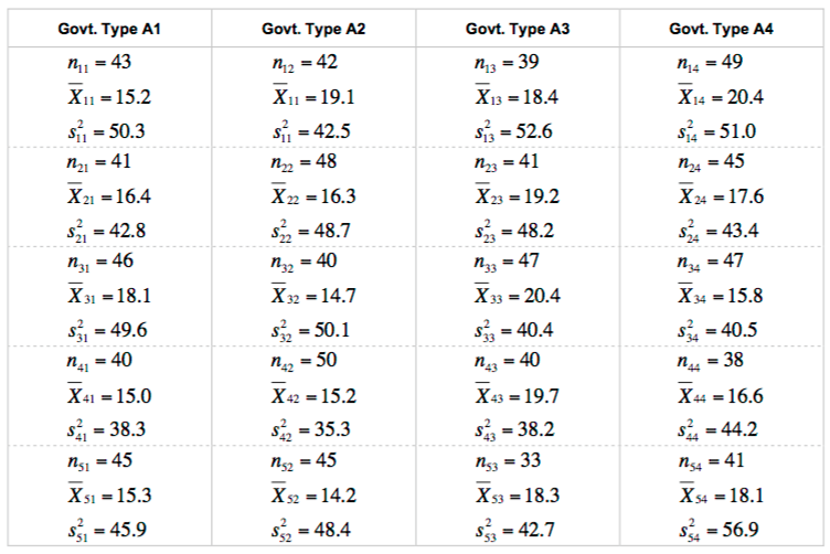
13. Notice the *stratified* random sampling technique used to select 5 communities and then 50 individuals within those communities. Do we have reason to believe the individuals (minor units) within each community (major unit) are similar to one another? In other words, do we believe there are dependencies within each community? Depending on your answers to the those questions, do we have 20 or 860 independent observations in this dataset? How many would we prefer to have?
This *Groups within Treatments* or (GwT ANOVA) design requires two separate analyses. First, we will begin under the hope that the 860 individuals in the study are independent observations. With this hope, we'll test to see if we find significant dependencies within each community. If we find significant dependencies, we'll need to re-run the analysis with only 20 independent observations.
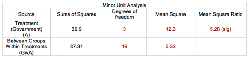
Here are the formulas we'd use to run the first *minor unit analysis*:
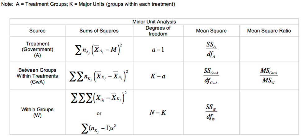
Our data would produce the following summary table. Note that weighted averages are used in all calculations (averages weighted by the number of individuals in each community):

If that mean square ratio were **not** statistically significant, we could treat all 860 individuals as independent observations and run a one-way ANOVA (with SSE = SSw + SSgwa).
Since the mean square ratio in this scenario produces a p-value less than 0.05, we may conclude that individuals within communities are **not** independent. Then we'd have to run a *major units analysis* using unweighted means (ignoring the sample size within each community):
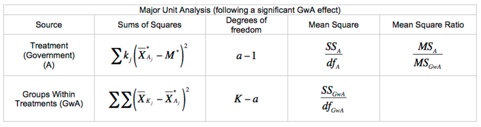
Here are the results from this dataset:
From this, we could conclude the types of governments are associated with different average levels of contentment.
*****
# Your turn
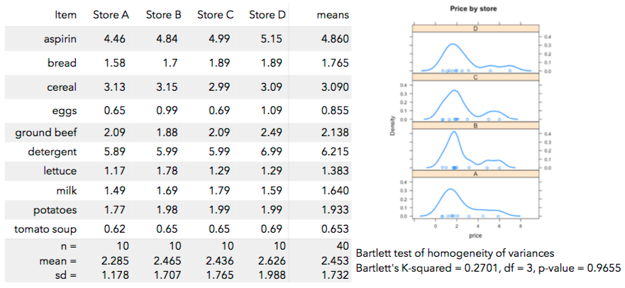
25. Do some stores charge higher prices than others for the same items? To study this, the prices of 10 items were found at 4 different stores. Conduct an AxS ANOVA to determine if mean prices differ across stores. To do this, do the following:
**(a)** Load the data and summarize it graphically and numerically.
**(b)** Run a one-way ANOVA (ignoring the fact that we have repeated measures) and state your conclusion.
**(c)** Sketch a profile plot of the prices across stores for each item.
**(d)** Run the AxS ANOVA and state your conclusions.
*****
# Publishing your solutions
When you're ready to try the **Your Turn** exercises:
- Download the appropriate [Your Turn file](http://bradthiessen.com/html5/M301.html).
- If the file downloads with a *.Rmd* extension, it should open automatically in RStudio.
- If the file downloads with a *.txt* extension (or if it does not open in RStudio), then:
- open the file in a text editor and copy its contents
- open RStudio and create a new **R Markdown** file (html file)
- paste the contents of the **Your Turn file** over the default contents of the R Markdown file.
- Type your solutions into the **Your Turn file**.
- The file attempts to show you *where* to type each of your solutions/answers.
- Once you're ready to publish your solutions, click the **Knit HTML** button located at the top of RStudio:  - Once you click that button, RStudio will begin working to create a .html file of your solutions.
- It may take a minute or two to compile everything, especially if your solutions contain simulation/randomization methods
- While the file is compiling, you may see some red text in the console.
- When the file is finished, it will open automatically.
- If the file does not open automatically, you'll see an error message in the console.
- Send me an [email](mailto:thiessenbradleya@sau.edu) with that error message and I should be able to help you out.
- Once you have a completed report of your solutions, look through it to see if everything looks ok. Then, send that yourturn.html file to me [via email](mailto:thiessenbradleya@sau.edu) or print it out and give it to me.
- Once you click that button, RStudio will begin working to create a .html file of your solutions.
- It may take a minute or two to compile everything, especially if your solutions contain simulation/randomization methods
- While the file is compiling, you may see some red text in the console.
- When the file is finished, it will open automatically.
- If the file does not open automatically, you'll see an error message in the console.
- Send me an [email](mailto:thiessenbradleya@sau.edu) with that error message and I should be able to help you out.
- Once you have a completed report of your solutions, look through it to see if everything looks ok. Then, send that yourturn.html file to me [via email](mailto:thiessenbradleya@sau.edu) or print it out and give it to me.
Sources:
This document is released under a [Creative Commons Attribution-ShareAlike 3.0 Unported](http://creativecommons.org/licenses/by-sa/3.0) license.